


Introduction
We will be making a MACHINE LEARNING model which predicts the price of a house taking different parameters into account.
We will be taking a house price dataset from Kaggle.com. The dataset has house prices of Bengaluru city. As we know that price of a house varies from area to area, so this model will be predicting price of Bengaluru city’s different areas and many other parameters into account.
While building the model we will go through different data science concepts such as Data cleaning and Outlier detection.
You can download the dataset from the following link: Dataset
We'll be using jupyter notebook as IDE
So let's get started!!🚀
First of all we will be importing the necessary libraries we need for this project:
import pandas as pd
import numpy as np
from matplotlib import pyplot as plt
%matplotlib inline
import matplotlib
matplotlib.rcParams["figure.figsize"] = (20,10)
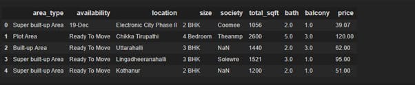
Now we will load our dataset that we just downloaded, then have a look at first five rows and the shape(number of rows and columns) of the csv file:
df1 = pd.read_csv("Bengaluru_House_Data.csv")
df1.head()
df1.shape

DATA CLEANING
Now we need to examine the dataset we have.
Data cleaning is important before feeding the dataset to our model as it can affect the accuracy of our model. So let’s see how we will do this.
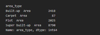
Let us have a look at count of each area type by grouping the data by area type:
df1.groupby('area_type')['area_type'].agg('count')
Now we know that not all the columns are necessary for prediction of the house price such as availability, society, area type. So let’s drop the columns which we think are not important:
df2 = df1.drop(['area_type', 'availability', 'society','balcony'],axis='columns')
df2.head()
We need to now drop the null values from the dataset that can affect the model while training.
df2.isnull().sum()
df3 = df2.dropna()
df3.isnull().sum()
The dataset shows BHK and Bedroom both in ‘size’ column.
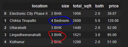 So we will create a new column named BHK which will show us the size of house in BHK particularly.
df3['size'].unique()
df3['bhk'] = df3['size'].apply(lambda x: int(x.split(' ')[0]))
df3.head()
df3['bhk'].unique()
df3[df3.bhk>20]
We have some houses with many bedrooms (like 43 BHK) and has comparatively less total_sqft which is practically difficult to believe.
There may be many like this so let’s perform some operations on total_sqft column.
df3['total_sqft'].unique()

def is_float(x):
    try:
        float(x)
    except:
        return False
    return True


df3[~df3['total_sqft'].apply(is_float)].head()
This shows that we have some values in total_sqft which are not certain, so we need to fix the uncertainities.
We will convert those ranges into average.
def convert_sqft_to_num(x):
    tokens = x.split('-')
    if len(tokens) == 2:
        return (float(tokens[0])+float(tokens[1]))/2
    try:
        return float(x)
    except:
        return None

df4 = df3.copy()
df4['total_sqft'] = df4['total_sqft'].apply(convert_sqft_to_num)
df4.head(3)
Now let’s create a column for price per sqft:
df5 = df4.copy()
df5['price_per_sqft'] = df5['price']*100000/df5['total_sqft']
df5.head()
Now let’s drop the location/area which have less entries, so that we can reduce our dimension and which are not important.
len(df5.location.unique())

df5.location = df5.location.apply(lambda x: x.strip())
location_stats = df5.groupby('location')['location'].agg('count').sort_values(ascending=False)
location_stats

len(location_stats[location_stats<10])

location_stats_less_than_10 = location_stats[location_stats<=10]
location_stats_less_than_10

len(df5.location.unique())

df5.location = df5.location.apply(lambda x: 'other' if x in location_stats_less_than_10 else x)
len(df5.location.unique())
df5.head(10)
OUTLIER REMOVAL
Now we will be detecting some outliers and eliminate them so that they don’t create any problem later on.
We will remove the rows which exceed the value of total sqft per bedroom than a particular threshold, because we can’t have more sqft per bedroom than that.
df5[df5.total_sqft/df5.bhk<300].head()
df6 = df5[~(df5.total_sqft/df5.bhk<300)]
df6.shape
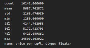
df6.price_per_sqft.describe()
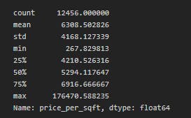 Now looking at the maximum and minimum
 price per sqft we cannot practically believe it.
As we are making a generic model, we can remove the price per sqft that are too low or too high.
def remove_pps_outliners(df):
    df_out = pd.DataFrame()
    for key,subdf in df.groupby('location'):
        m = np.mean(subdf.price_per_sqft)
        st = np.std(subdf.price_per_sqft)
        reduced_df = subdf[(subdf.price_per_sqft>(m-st)) & (subdf.price_per_sqft<(m+st))]
        df_out = pd.concat([df_out,reduced_df],ignore_index=True)
    return df_out
df7 = remove_pps_outliners(df6)
df7.shape

df7.head()

df7.price_per_sqft.describe()
 Now this makes some sense right?
def plot_scatter_chart(df,location):
    bhk2 = df[(df.location == location) & (df.bhk == 2)]
    bhk3 = df[(df.location == location) & (df.bhk == 3)]
    matplotlib.rcParams['figure.figsize'] = (15,10)
    plt.scatter(bhk2.total_sqft,bhk2.price, color='blue',label='2 BHK', s=50)
    plt.scatter(bhk3.total_sqft, bhk3.price, marker='+', color='green', label='3 BHK', s = 50)
    plt.xlabel("Total Square Feet Area")
    plt.ylabel("Price")
    plt.title("Location")
    plt.show()

plot_scatter_chart(df7, "Hebbal")
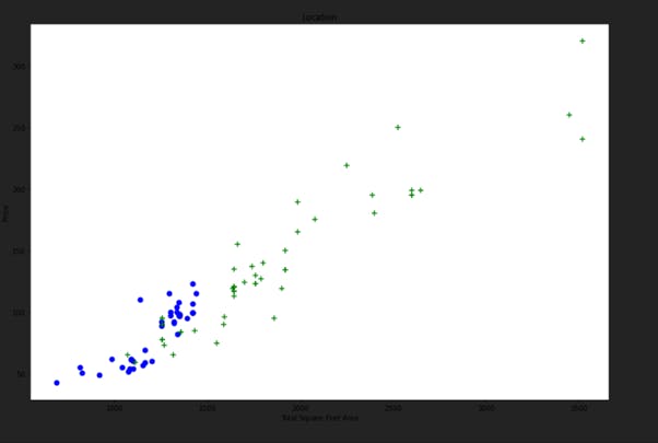 The function takes a dataframe and the location as parameter and plots a TOTAL_SQFT_AREA VS PRICE graph for us.
The blue dots represent 2BHK house price of a particular area and green marker represents 3BHK house price of the same area.
We see that some 3BHK flats have less price than 2BHK flats even they are in same area.
So we need to eliminate such Outliers.
We will remove those (N)bhk appartments whose price per sqft is less than mean price per sqft of (N-1)bhk apartment.
def remove_bhk_outliers(df):
    exclude_indices = np.array([])
    for location , location_df in df.groupby('location'):
            bhk_stats = {}
            for bhk, bhk_df in location_df.groupby('bhk'):
                bhk_stats[bhk] = {
                    'mean' : np.mean(bhk_df.price_per_sqft),
                    'std' : np.std(bhk_df.price_per_sqft),
                    'count' : bhk_df.shape[0]
                }
            for bhk, bhk_df in location_df.groupby('bhk'):
                stats = bhk_stats.get(bhk-1)
                if stats and stats['count']>5:
                    exclude_indices = np.append(exclude_indices, bhk_df[bhk_df.price_per_sqft<(stats['mean'])].index.values)
    return df.drop(exclude_indices,axis='index')

df8 = remove_bhk_outliers(df7)
df8.shape


plot_scatter_chart(df8, "Hebbal")
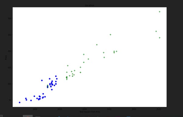 Now let us detect and remove some more outliers.
plt.hist(df8.bath,rwidth=0.8)
plt.xlabel("Number of bathrooms")
plt.ylabel("Count")

df8[df8.bath>df8.bhk+2]

df9 = df8[df8.bath<df8.bhk+2]
df9.shape

df10 = df9.drop(['size','price_per_sqft'],axis='columns')
df10.head(10)
Now we need to convert the categorical information(location column) into numerical information.
We will do it using dummies.
dummies = pd.get_dummies(df10.location)
dummies.head(3)
df11 = pd.concat([df10,dummies.drop('other',axis='columns')],axis='columns')
df11.head(3)

df12 = df11.drop('location',axis='columns')
df12.head()
df12.shape
MODEL TRAINING
So let's finally get started with training our model 😋.
We will get all feature columns in X and the target column price in y.
X = df12.drop('price',axis='columns')
X.head()
y = df12.price
y.head()
Now we will Split the dataframe in training set and test set using sklearn
from sklearn.model_selection import train_test_split
X_train, X_test, y_train, y_test = train_test_split(X,y,test_size=0.2,random_state=10)
We will now create a linear regression. model and call the fit method on X_train and y_train and then evaluate the score of our model.
from sklearn.linear_model import LinearRegression
lr_clf = LinearRegression()
lr_clf.fit(X_train,y_train)
lr_clf.score(X_test,y_test)
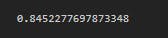 We get an accuracy of 84% but we want to look for optimal model, so we will use k-fold cross validation . So we will use different sets of X_train and y_train.
from sklearn.model_selection import ShuffleSplit
from sklearn.model_selection import cross_val_score

cv = ShuffleSplit(n_splits=5, test_size=0.2, random_state=0)
cross_val_score(LinearRegression(),X,y,cv=cv)
 We get more than 80% of accuracy majority of the time.
You can use different regression techniques on this dataset and find out which can be the best algorithm. There are different regression techniques like lasso regression which you can use and find out the model with best accuracy.
We can use Grid search cv.
from sklearn.model_selection import GridSearchCV

from sklearn.linear_model import Lasso
from sklearn.tree import DecisionTreeRegressor

def find_best_model_using_gridsearchcv(X,y):
    algos = {
        'linear_regression' : {
            'model': LinearRegression(),
            'params': {
                'normalize': [True, False]
            }
        },
        'lasso': {
            'model': Lasso(),
            'params': {
                'alpha': [1,2],
                'selection': ['random', 'cyclic']
            }
        },
        'decision_tree': {
            'model': DecisionTreeRegressor(),
            'params': {
                'criterion' : ['mse','friedman_mse'],
                'splitter': ['best','random']
            }
        }
    }
    scores = []
    cv = ShuffleSplit(n_splits=5, test_size=0.2, random_state=0)
    for algo_name, config in algos.items():
        gs =  GridSearchCV(config['model'], config['params'], cv=cv, return_train_score=False)
        gs.fit(X,y)
        scores.append({
            'model': algo_name,
            'best_score': gs.best_score_,
            'best_params': gs.best_params_
        })

    return pd.DataFrame(scores,columns=['model','best_score','best_params'])

find_best_model_using_gridsearchcv(X,y)
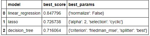
Now we will make a function and test the model which will help us predict the house price.
def predict_price(location,sqft,bath,bhk):
    loc_index=np.where(X.columns == location)[0][0]

    x=np.zeros(len(X.columns))
    x[0] = sqft
    x[1] = bath
    x[2] = bhk
    if loc_index >=0:
        x[loc_index] = 1
    return lr_clf.predict([x])[0]
Now let us predict the price using our model
predict_price('1st Phase JP Nagar',1000,2,2)

predict_price('Indira Nagar',1000,3,3)
So in a similar way, you can create a model for predicting house price of all over india using a different dataset.
If you find this blog helpful then please give it a like..😊
Thanks for reading!!